Removing scattered light from TESS light curves using linear regression (RegressionCorrector)#
Learning Goals#
By the end of this tutorial, you will: - Be familiar with the Lightkurve RegressionCorrector. - Understand how to create regressors from a TargetPixelFile object. - Be able to remove the scattered light background signal from TESS data.
Introduction#
Lightkurve offers several tools to the community for removing instrument noise and systematics from data from the Kepler, K2, and TESS missions. This tutorial will demonstrate the use of Lightkurve’s RegressionCorrector class to remove the scattered light and spacecraft motion noise from TESS Full Frame Images (FFIs).
TESS FFIs have an additive scattered light background that has not been removed by the pipeline. This scattered light must be removed by the user. This can be done in a few ways, including a basic median subtraction. In this tutorial, we’ll show you how to use Lightkurve’s corrector tools to remove the scattered light.
Imports#
This tutorial requires the Lightkurve package, and also makes use of NumPy and Matplotlib.
[1]:
import lightkurve as lk
import numpy as np
import matplotlib.pyplot as plt
%matplotlib inline
1. Using RegressionCorrector on TESSCut FFI Cutouts#
For this tutorial we will use the TESS Sector 15 data of KIC 8462852 (also known as Boyajian’s Star). We’ll start by downloading the FFI data using MAST’s TESSCut service, querying it through Lightkurve.
[2]:
target = "KIC 8462852"  # Boyajian's Star
tpf = lk.search_tesscut(target, sector=15).download(cutout_size=(50, 50))
[3]:
tpf
[3]:
TessTargetPixelFile(TICID: KIC 8462852)
This cutout works the same as any Lightkurve target pixel file (TPF). TESS FFI cutouts do not have aperture masks created by the pipeline. Instead, users must create their own apertures. There are many methods we could use to do this, but for now we can create a threshold aperture, using Lightkurve’s create_threshold_mask() method.
[4]:
aper = tpf.create_threshold_mask()
Let’s plot the aperture to make sure it selected the star in the center and has a reasonable number of pixels.
[5]:
tpf.plot(aperture_mask=aper);
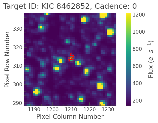
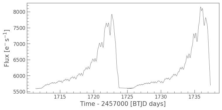
Looks good. We can sum up the pixels in this aperture, and create an uncorrected light curve.
[6]:
uncorrected_lc = tpf.to_lightcurve(aperture_mask=aper)
[7]:
uncorrected_lc.plot();
2. Creating a DesignMatrix from Pixel Regressors#
The flux in the aperture appears to be dominated by scattered light. We can tell because TESS orbits Earth twice in each sector, thus patterns which appear twice within a sector are typically related to the TESS orbit (such as the scattered light effect).
To remove this light, we are going to detrend the light curve against some vectors which we think are predictive of this systematic noise.
In this case, we can use the pixels outside the aperture as vectors that are highly predictive of the systematic noise, that is, we will make the assumption that these pixels do not contain any flux from our target.
We can select these pixels by specifying flux outside of the aperture using Python’s bitwise invert operator ~ to take the inverse of the aperture mask.
[8]:
regressors = tpf.flux[:, ~aper]
[9]:
regressors.shape
[9]:
(1190, 2491)
regressors is now an array with shape ntime x npixels outside of the aperture. If we plot the first 30 of these pixels, we can see that they contain mostly scattered light, with some offset terms.
[10]:
plt.plot(regressors[:, :30]);

In linear regression problems, it is common to refer to the matrix of regressors as the design matrix (also known as model matrix or regressor matrix). Lightkurve provides a convenient DesignMatrix class which is designed to help you work with detrending vectors.
The DesignMatrix class has several convenience functions, and can be passed into Lightkurve’s corrector objects.
[11]:
from lightkurve.correctors import DesignMatrix
dm = DesignMatrix(regressors, name='regressors')
[12]:
dm
[12]:
regressors DesignMatrix (1190, 2491)
As shown above, dm is now a design matrix with the same shape as the input pixels. Currently, we have 2,541 pixels that we are using to detrend our light curve against. Rather than using all of the pixels, we can reduce these to their principal components using Principal Component Analysis (PCA). We do this for several reasons:
By reducing to a smaller number of vectors, we can remove some of the stochastic noise in our detrending vectors.
By reducing to the principal components, we can avoid pixels that have intrinsic variability (for example, from astrophysical long-period variables) that can be confused with the true astrophysical signal of our target.
By reducing the number of vectors, our detrending will be faster (although in this case, the detrending will still take seconds).
The choice of the number of components is a tricky issue, but in general you should choose a number that is much smaller than the number of vectors.
[13]:
dm = dm.pca(5)
[14]:
dm
[14]:
regressors DesignMatrix (1190, 5)
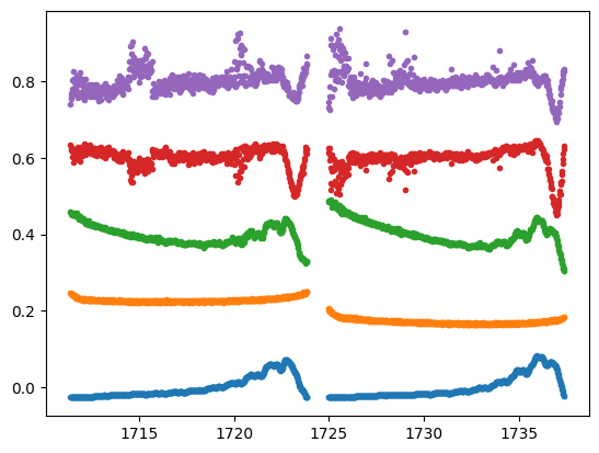
Using the pca() method, we have now reduced the number of components in our design matrix to five. These vectors show a combination of scattered light and spacecraft motion, which makes them suited to detrend our input light curve.
[15]:
plt.plot(tpf.time.value, dm.values + np.arange(5)*0.2, '.');
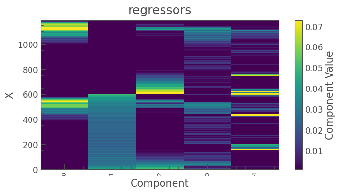
Note: the DesignMatrix object provides a convenient plot() method to visualize the vectors:
[16]:
dm.plot();
We can now detrend the uncorrected light curve against these vectors. Lightkurve’s RegressionCorrector will use linear algebra to find the combination of vectors that makes the input light curve closest to zero. To do this, we need one more component; we need an “offset” term, to be able to fit the mean level of the light curve. We can do this by appending a “constant” to our design matrix.
[17]:
dm = dm.append_constant()
3. Removing Background Scattered Light Using Linear Regression#
Now that we have a design matrix, we only need to pass it into a lightkurve.Corrector. To use our design matrix, we can pass it to the RegressionCorrector, which will detrend the input light curve against the vectors we’ve built.
[18]:
from lightkurve.correctors import RegressionCorrector
corrector = RegressionCorrector(uncorrected_lc)
[19]:
corrector
[19]:
RegressionCorrector (ID: KIC 8462852)
To correct the light curve, we pass in our design matrix.
[20]:
corrected_lc = corrector.correct(dm)
Now we can plot the results:
[21]:
ax = uncorrected_lc.plot(label='Original light curve')
corrected_lc.plot(ax=ax, label='Corrected light curve');
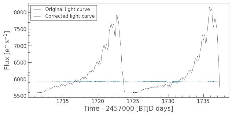
As shown above, the scattered light from the background has been removed. If we want to take a more in-depth look at the correction, we can use the diagnose() method to see what the RegressionCorrector found as the best fitting solution.
4. Diagnosing the Correction#
[22]:
corrector.diagnose();
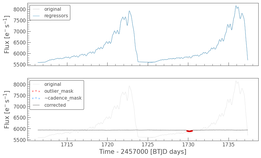
The RegressionCorrector has clipped out some outliers during the fit of the trend. You can read more about the outlier removal, how to pass a cadence mask, and error propagation in the docs.
Watch Out!
The RegressionCorrector assumes that you want to remove the trend and set the light curve to the mean level of the uncorrected light curve. This isn’t true for TESS scattered light. TESS FFI light curves have additive background, and so we want to reduce the flux to the lowest recorded level, assuming that at that point the contribution from scattered light is approximately zero.
To do this, we will first need to look at the model of the background that RegressionCorrector built. We can access that in the corrector object.
[23]:
corrector.model_lc
[23]:
| time | flux | flux_err |
|---|---|---|
| electron / s | electron / s | |
| Time | float64 | float64 |
| 1711.3882446289062 | -341.18816068932574 | 0.0 |
| 1711.4090576171875 | -341.21407886444376 | 0.0 |
| 1711.4298706054688 | -341.9634439703268 | 0.0 |
| 1711.4507446289062 | -341.83822804044485 | 0.0 |
| 1711.4715576171875 | -342.1986575923647 | 0.0 |
| 1711.4923706054688 | -342.1091946304241 | 0.0 |
| ... | ... | ... |
| 1737.2837524414062 | 218.35482253288046 | 0.0 |
| 1737.3045654296875 | 109.6059244113103 | 0.0 |
| 1737.3253784179688 | 2.488369893856543 | 0.0 |
| 1737.3462524414062 | -92.91965046689711 | 0.0 |
| 1737.3670654296875 | -179.75423736150879 | 0.0 |
| 1737.3878784179688 | -238.60812425258882 | 0.0 |
[24]:
model = corrector.model_lc
model.plot();
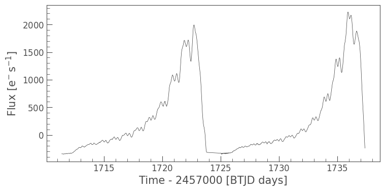
As you can see above, the model drops below zero flux. This is impossible; the scattered light can’t be removing flux from our target!
To rectify this, we can subtract the model flux value at the 5th percentile.
[25]:
# Normalize to the 5th percentile of model flux
model -= np.percentile(model.flux, 5)
[26]:
model.plot();
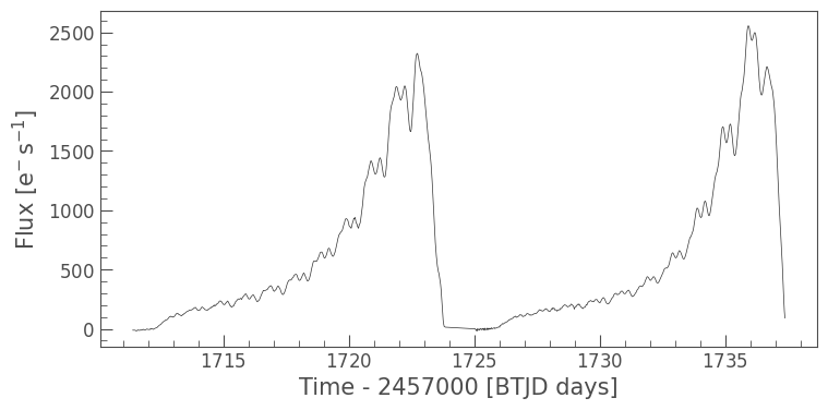
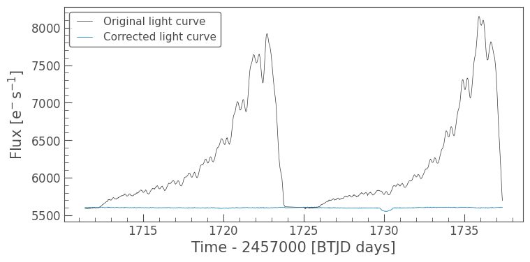
This looks better. Now we can remove this model from our uncorrected light curve.
[27]:
corrected_lc = uncorrected_lc - model
[28]:
ax = uncorrected_lc.plot(label='Original light curve')
corrected_lc.plot(ax=ax, label='Corrected light curve');

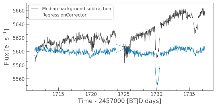
This looks great. As a final test, let’s investigate how the light curve we obtained using RegressionCorrector compares against a light curve obtained using a more basic median background removal method.
[29]:
bkg = np.median(regressors, axis=1)
bkg -= np.percentile(bkg, 5)

npix = aper.sum()
median_subtracted_lc = uncorrected_lc - npix * bkg

ax = median_subtracted_lc.plot(label='Median background subtraction')
corrected_lc.plot(ax=ax, label='RegressionCorrector');
Lastly, let’s show how you can do all of the above in a single cell.
[30]:
# Make an aperture mask and an uncorrected light curve
aper = tpf.create_threshold_mask()
uncorrected_lc = tpf.to_lightcurve(aperture_mask=aper)

# Make a design matrix and pass it to a linear regression corrector
dm = DesignMatrix(tpf.flux[:, ~aper], name='regressors').pca(5).append_constant()
rc = RegressionCorrector(uncorrected_lc)
corrected_ffi_lc = rc.correct(dm)

# Optional: Remove the scattered light, allowing for the large offset from scattered light
corrected_ffi_lc = uncorrected_lc - rc.model_lc + np.percentile(rc.model_lc.flux, 5)
[31]:
ax = uncorrected_lc.plot(label='Original light curve')
corrected_ffi_lc.plot(ax=ax, label='Corrected light curve');
5. Using RegressionCorrector on TESS Two-Minute Cadence Target Pixel Files#
TESS releases high-time resolution TPFs of interesting targets. These higher time resolution TPFs have background removed for users by the pipeline. However, there are still common trends in TPF pixels that are not due to scattered light, but could be from, for example, spacecraft motion.
RegressionCorrector can be used in exactly the same way to remove these common trends.
[32]:
# Download a 2-minute cadence Target Pixel File (TPF)
tpf_2min = lk.search_targetpixelfile(target, author='SPOC', cadence=120, sector=15).download()
[33]:
tpf_2min
[33]:
TessTargetPixelFile(TICID: 185336364)
Note, unlike the FFI data, the TPF has been processed by the SPOC pipeline, and includes an aperture mask.
[34]:
# Use the pipeline aperture and an uncorrected light curve
aper = tpf_2min.pipeline_mask
uncorrected_lc = tpf_2min.to_lightcurve()

# Make a design matrix
dm = DesignMatrix(tpf_2min.flux[:, ~aper], name='pixels').pca(5).append_constant()

# Regression Corrector Object
reg = RegressionCorrector(uncorrected_lc)
corrected_lc = reg.correct(dm)
[35]:
ax = uncorrected_lc.errorbar(label='Original light curve')
corrected_lc.errorbar(ax=ax, label='Corrected light curve');
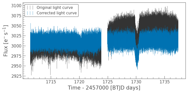
As you can see, the corrected light curve has removed long-term trends and some motion noise, for example, see time around 1720 Barycentric TESS Julian Date (BTJD). We can use the same diagnose() method to understand the model that has been fit and subtracted by RegressionCorrector.
[36]:
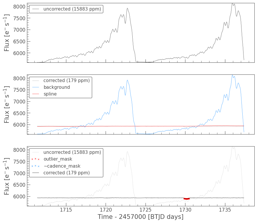
reg.diagnose();
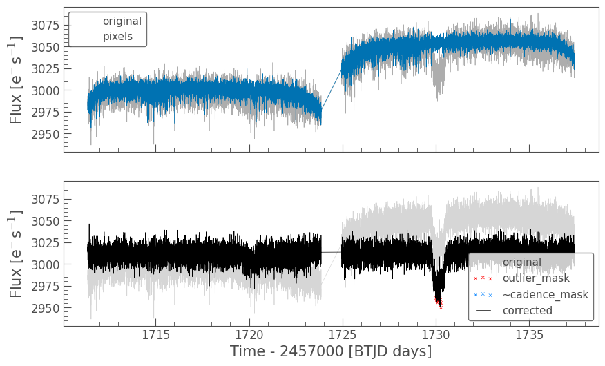
To show the corrected version has improved, we can use the Combined Differential Photometric Precision (CDPP) metric. As shown below, the corrected light curve has a lower CDPP, showing it is less noisy.
[37]:
uncorrected_lc.estimate_cdpp()
[37]:
[38]:
corrected_lc.estimate_cdpp()
[38]:
6. Should I use RegressionCorrector or PLDCorrector?#
In addition to the corrector demonstrated in this tutorial, Lightkurve has a special case of RegressionCorrector called PLDCorrector. PLD, or Pixel Level Decorrelation, is a method of removing systematic noise from light curves using linear regression, with a design matrix constructed from a combination of pixel-level light curves.
For more information about the PLDCorrector, please see the tutorial specifically on removing instrumental noise from K2 and TESS light curves using PLD.
For TESS, the PLDCorrector works in a very similar way to the RegressionCorrector. The major difference between them is that PLDCorrector constructs its own design matrix, making it a streamlined, versatile tool to apply to any TESS or K2 light curve.
Here, we perform PLD and diagnose the correction in just three lines. To make a more direct comparison to the RegressionCorrector, we pass in arguments to set the number of components to five (as in section 2), as well as remove the spline fit.
[39]:
from lightkurve.correctors import PLDCorrector
pld = PLDCorrector(tpf)
pld_corrected_lc = pld.correct(restore_trend=False, pca_components=5)
pld.diagnose();
And there we go!
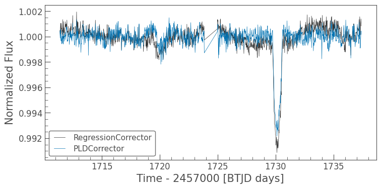
Now let’s compare the performance of these two corrections.
[40]:
ax = corrected_ffi_lc.normalize().plot(label='RegressionCorrector')
pld_corrected_lc.normalize().plot(label='PLDCorrector', ax=ax);
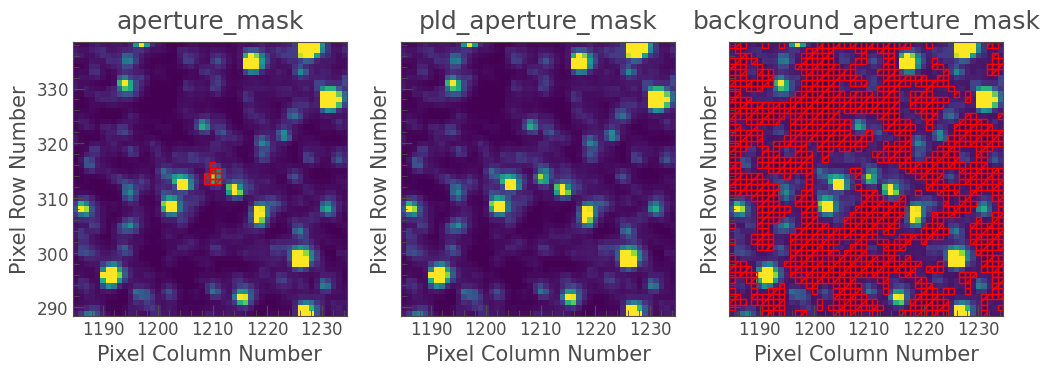
PLDCorrector offers an additional diagnostic plot, named diagnose_masks. This allows you to inspect the pixels that were used to create your design matrix.
[41]:
pld.diagnose_masks();
While it is more convenient to apply to light curves and generally works well with default parameters, the PLDCorrector is less flexible than the RegressionCorrector, which allows you to create your own custom design matrix. However, the PLDCorrector also allows you to create “higher order” PLD regressors by taking the products of existing pixel regressors, which improves the performance of corrections to K2 data (see the paper by Luger et al.
2016 for more information).
When considering which corrector to use, remember that PLDCorrector is minimal and designed to be effective at removing both background scattered light from TESS and motion noise from K2, while RegressionCorrector is flexible and gives you more control over the creation of the design matrix and the correction.
About this Notebook#
Authors: Christina Hedges (christinalouisehedges@gmail.com), Nicholas Saunders (nksaun@hawaii.edu), Geert Barentsen
Updated On: 2020-09-28
Citing Lightkurve and its Dependencies#
If you use lightkurve or its dependencies for published research, please cite the authors. Click the buttons below to copy BibTeX entries to your clipboard.
[42]:
lk.show_citation_instructions()
[42]:
When using Lightkurve, we kindly request that you cite the following packages:
- lightkurve
- astropy
- astroquery — if you are using search_lightcurve() or search_targetpixelfile().
- tesscut — if you are using search_tesscut().
