Combining multiple quarters of Kepler data#
Learning Goals#
By the end of this tutorial, you will:
Understand a Kepler Quarter.
Understand how to download multiple quarters of data at once.
Learn how to normalize Kepler data.
Understand how to combine multiple quarters of data.
Introduction#
The Kepler, K2, and TESS telescopes observe stars for long periods of time. These long, time series observations are broken up into separate chunks, called quarters for the Kepler mission, campaigns for K2, and sectors for TESS.
Building light curves with as much data as is available is useful when searching for small signals, such as planetary transits or stellar pulsations. In this tutorial, we will learn how to use Lightkurve’s tools to download and stitch together multiple quarters of Kepler observations.
It is recommended to first read the tutorial discussing how to use Kepler light curve products with Lightkurve. That tutorial will introduce you to some specifics of how Kepler, K2, and TESS make observations, and how these are displayed as light curves. It also introduces some important terms and concepts that are referred to in this tutorial.
This tutorial demonstrates how to access and combine multiple quarters of data from the Kepler space telescope, using the Lightkurve package.
When accessing Kepler data through MAST, it will be stored in three-month chunks, corresponding to a quarter of observations. By combining and normalizing these separate observations, you can form a single light curve that spans all observed quarters. Utilizing all of the data available is especially important when looking at repeating signals, such as planet transits and stellar oscillations.
We will use the Kepler mission as an example, but these tools are extensible to TESS and K2 as well.
Imports#
This tutorial requires the Lightkurve package, which in turn uses matplotlib for plotting.
[1]:
import lightkurve as lk
%matplotlib inline
1. What is a Kepler Quarter?#
In order to search for planets around other stars, the Kepler space telescope performed near-continuous monitoring of a single field of view, from an Earth-trailing orbit. However, this posed a challenge. If the space telescope is trailing Earth and maintaining steady pointing, its solar panels would slowly receive less and less sunlight.
In order to make sure the solar panels remained oriented towards the Sun, Kepler performed quarterly rolls, one every 93 days. The infographic below helps visualize this, and shows the points in the orbit where the rolls took place.
After each roll, Kepler retained its fine-pointing at the same field of view. Because the camera rotated by 90 degrees, all of the target stars fell on different parts of the charge-coupled device (CCD) camera. This had an effect on the amount of flux recorded for the same star, because different CCD pixels have different sensitivities. The way in which the flux from the same stars was distributed on the CCD (called the point spread function or PSF) also changed after each roll, due to focus changes and other instrumental effects. As a result, the aperture mask set for a star had to be recomputed after each roll, and may capture slightly different amounts of flux.
The data obtained between rolls is referred to as a quarter. While there are changes to the flux systematics, not much else changes quarter to quarter, and the majority of the target list remains identical. This means that, after removing systematic trends (such as was done for the presearch data conditioning simple aperture photometry (PDCSAP) flux), multiple quarters together can form one continuous observation.

Figure: Infographic showcasing the necessity of Kepler’s quarterly rolls and its Earth-trailing orbit. Source: Kepler Science Center.
Note: Observations by K2 and TESS are also broken down into chunks of a month or more, called campaigns (for K2) and sectors (for TESS). While not discussed in this tutorial, the tools below work for these data products as well.
2. Downloading Multiple KeplerLightCurve Objects at Once#
To start, we can use Lightkurve’s search_lightcurve() function to see what data are available for our target star on the Mikulski Archive for Space Telescopes (MAST) archive. We will use the star Kepler-8, a star somewhat larger than the Sun, and the host of a hot Jupiter planet.
[2]:
search_result = lk.search_lightcurve("Kepler-8", author="Kepler", cadence="long")
search_result
[2]:
| # | mission | year | author | exptime | target_name | distance |
|---|---|---|---|---|---|---|
| s | arcsec | |||||
| 0 | Kepler Quarter 00 | 2009 | Kepler | 1800 | kplr006922244 | 0.0 |
| 1 | Kepler Quarter 01 | 2009 | Kepler | 1800 | kplr006922244 | 0.0 |
| 2 | Kepler Quarter 02 | 2009 | Kepler | 1800 | kplr006922244 | 0.0 |
| 3 | Kepler Quarter 03 | 2009 | Kepler | 1800 | kplr006922244 | 0.0 |
| 4 | Kepler Quarter 04 | 2010 | Kepler | 1800 | kplr006922244 | 0.0 |
| 5 | Kepler Quarter 05 | 2010 | Kepler | 1800 | kplr006922244 | 0.0 |
| ... | ... | ... | ... | ... | ... | ... |
| 11 | Kepler Quarter 11 | 2012 | Kepler | 1800 | kplr006922244 | 0.0 |
| 12 | Kepler Quarter 12 | 2012 | Kepler | 1800 | kplr006922244 | 0.0 |
| 13 | Kepler Quarter 13 | 2012 | Kepler | 1800 | kplr006922244 | 0.0 |
| 14 | Kepler Quarter 14 | 2012 | Kepler | 1800 | kplr006922244 | 0.0 |
| 15 | Kepler Quarter 16 | 2013 | Kepler | 1800 | kplr006922244 | 0.0 |
| 16 | Kepler Quarter 15 | 2013 | Kepler | 1800 | kplr006922244 | 0.0 |
| 17 | Kepler Quarter 17 | 2013 | Kepler | 1800 | kplr006922244 | 0.0 |
In this list, each row represents a different observing quarter, for a total of 18 quarters across four years. The observation column lists the Kepler Quarter. The target_name represents the Kepler Input Catalogue (KIC) ID of the target, and the productFilename column is the name of the FITS files downloaded from MAST. The distance column shows the separation on the sky between the searched coordinates and the downloaded objects — this is only relevant when searching for specific coordinates in the sky, and not when looking for individual objects.
Instead of downloading a single quarter using the download() function, we can use the download_all() function to access all 18 quarters at once (this might take a while).
[3]:
lc_collection = search_result.download_all()
lc_collection
[3]:
LightCurveCollection of 18 objects:
    0: <KeplerLightCurve LABEL="KIC 6922244" QUARTER=0 AUTHOR=Kepler FLUX_ORIGIN=pdcsap_flux>
    1: <KeplerLightCurve LABEL="KIC 6922244" QUARTER=1 AUTHOR=Kepler FLUX_ORIGIN=pdcsap_flux>
    2: <KeplerLightCurve LABEL="KIC 6922244" QUARTER=2 AUTHOR=Kepler FLUX_ORIGIN=pdcsap_flux>
    3: <KeplerLightCurve LABEL="KIC 6922244" QUARTER=3 AUTHOR=Kepler FLUX_ORIGIN=pdcsap_flux>
    4: <KeplerLightCurve LABEL="KIC 6922244" QUARTER=4 AUTHOR=Kepler FLUX_ORIGIN=pdcsap_flux>
    5: <KeplerLightCurve LABEL="KIC 6922244" QUARTER=5 AUTHOR=Kepler FLUX_ORIGIN=pdcsap_flux>
    6: <KeplerLightCurve LABEL="KIC 6922244" QUARTER=6 AUTHOR=Kepler FLUX_ORIGIN=pdcsap_flux>
    7: <KeplerLightCurve LABEL="KIC 6922244" QUARTER=7 AUTHOR=Kepler FLUX_ORIGIN=pdcsap_flux>
    8: <KeplerLightCurve LABEL="KIC 6922244" QUARTER=10 AUTHOR=Kepler FLUX_ORIGIN=pdcsap_flux>
    9: <KeplerLightCurve LABEL="KIC 6922244" QUARTER=8 AUTHOR=Kepler FLUX_ORIGIN=pdcsap_flux>
    10: <KeplerLightCurve LABEL="KIC 6922244" QUARTER=9 AUTHOR=Kepler FLUX_ORIGIN=pdcsap_flux>
    11: <KeplerLightCurve LABEL="KIC 6922244" QUARTER=11 AUTHOR=Kepler FLUX_ORIGIN=pdcsap_flux>
    12: <KeplerLightCurve LABEL="KIC 6922244" QUARTER=12 AUTHOR=Kepler FLUX_ORIGIN=pdcsap_flux>
    13: <KeplerLightCurve LABEL="KIC 6922244" QUARTER=13 AUTHOR=Kepler FLUX_ORIGIN=pdcsap_flux>
    14: <KeplerLightCurve LABEL="KIC 6922244" QUARTER=14 AUTHOR=Kepler FLUX_ORIGIN=pdcsap_flux>
    15: <KeplerLightCurve LABEL="KIC 6922244" QUARTER=16 AUTHOR=Kepler FLUX_ORIGIN=pdcsap_flux>
    16: <KeplerLightCurve LABEL="KIC 6922244" QUARTER=15 AUTHOR=Kepler FLUX_ORIGIN=pdcsap_flux>
    17: <KeplerLightCurve LABEL="KIC 6922244" QUARTER=17 AUTHOR=Kepler FLUX_ORIGIN=pdcsap_flux>
All of the downloaded data are stored in a LightCurveCollection. This object acts as a wrapper for 18 separate KeplerLightCurve objects, listed above.
We can access the KeplerLightCurve objects and interact with them as usual through the LightCurveCollection.
[4]:
lc_Q4 = lc_collection[4]
lc_Q4
[4]:
| time | flux | flux_err | quality | timecorr | centroid_col | centroid_row | cadenceno | sap_flux | sap_flux_err | sap_bkg | sap_bkg_err | pdcsap_flux | pdcsap_flux_err | sap_quality | psf_centr1 | psf_centr1_err | psf_centr2 | psf_centr2_err | mom_centr1 | mom_centr1_err | mom_centr2 | mom_centr2_err | pos_corr1 | pos_corr2 |
|---|---|---|---|---|---|---|---|---|---|---|---|---|---|---|---|---|---|---|---|---|---|---|---|---|
| electron / s | electron / s | d | pix | pix | electron / s | electron / s | electron / s | electron / s | electron / s | electron / s | pix | pix | pix | pix | pix | pix | pix | pix | pix | pix | ||||
| Time | float32 | float32 | int32 | float32 | float64 | float64 | int32 | float32 | float32 | float32 | float32 | float32 | float32 | int32 | float64 | float32 | float64 | float32 | float64 | float32 | float64 | float32 | float32 | float32 |
| 352.37632485035283 | ——— | ——— | 0 | -1.410670e-03 | 682.69125 | 190.13296 | 11914 | 4.3689148e+04 | 6.6459765e+00 | 1.6722699e+03 | 4.6767941e-01 | ——— | ——— | 0 | 682.60927 | 7.8001787e-05 | 190.36814 | 1.1752916e-04 | 682.69125 | 1.8638317e-04 | 190.13296 | 1.8306405e-04 | 9.8764673e-02 | -1.7217098e-01 |
| 352.3967580484896 | 5.2490750e+04 | 8.0003128e+00 | 10000000000000 | -1.411072e-03 | 682.69084 | 190.13270 | 11915 | 4.3698070e+04 | 6.6462421e+00 | 1.6698400e+03 | 4.6764868e-01 | 5.2490750e+04 | 8.0003128e+00 | 10000000000000 | 682.60900 | 7.7997785e-05 | 190.36777 | 1.1751152e-04 | 682.69084 | 1.8633612e-04 | 190.13270 | 1.8303936e-04 | 9.8700106e-02 | -1.7229939e-01 |
| 352.4376244455707 | 5.2484055e+04 | 7.9999790e+00 | 10000 | -1.411874e-03 | 682.69038 | 190.13302 | 11917 | 4.3694105e+04 | 6.6461620e+00 | 1.6731306e+03 | 4.6705514e-01 | 5.2484055e+04 | 7.9999790e+00 | 10000 | 682.60862 | 7.7994831e-05 | 190.36848 | 1.1754913e-04 | 682.69038 | 1.8634219e-04 | 190.13302 | 1.8301954e-04 | 9.8306537e-02 | -1.7180158e-01 |
| 352.45805764463876 | 5.2491809e+04 | 8.0006199e+00 | 0 | -1.412275e-03 | 682.69084 | 190.13257 | 11918 | 4.3698316e+04 | 6.6463132e+00 | 1.6741406e+03 | 4.6687824e-01 | 5.2491809e+04 | 8.0006199e+00 | 0 | 682.60872 | 7.7998680e-05 | 190.36792 | 1.1751390e-04 | 682.69084 | 1.8635279e-04 | 190.13257 | 1.8304381e-04 | 9.8410256e-02 | -1.7202987e-01 |
| 352.4784908439324 | 5.2478277e+04 | 7.9992733e+00 | 0 | -1.412676e-03 | 682.68949 | 190.13304 | 11919 | 4.3687648e+04 | 6.6459165e+00 | 1.6723815e+03 | 4.6764576e-01 | 5.2478277e+04 | 7.9992733e+00 | 0 | 682.60829 | 7.7993544e-05 | 190.36814 | 1.1756293e-04 | 682.68949 | 1.8641398e-04 | 190.13304 | 1.8308057e-04 | 9.8039381e-02 | -1.7183834e-01 |
| 352.4989240434661 | 5.2475855e+04 | 7.9986620e+00 | 0 | -1.413077e-03 | 682.69036 | 190.13318 | 11920 | 4.3686480e+04 | 6.6458707e+00 | 1.6734375e+03 | 4.6817183e-01 | 5.2475855e+04 | 7.9986620e+00 | 0 | 682.60852 | 7.7998702e-05 | 190.36875 | 1.1761812e-04 | 682.69036 | 1.8637831e-04 | 190.13318 | 1.8304847e-04 | 9.8102726e-02 | -1.7151666e-01 |
| ... | ... | ... | ... | ... | ... | ... | ... | ... | ... | ... | ... | ... | ... | ... | ... | ... | ... | ... | ... | ... | ... | ... | ... | ... |
| 442.1013323661464 | 5.2484648e+04 | 7.9707704e+00 | 0 | -3.378539e-04 | 682.49086 | 190.34446 | 16305 | 4.3164066e+04 | 6.6142449e+00 | 1.4996798e+03 | 4.6686992e-01 | 5.2484648e+04 | 7.9707704e+00 | 0 | 682.42295 | 7.3321760e-05 | 190.68497 | 9.3209848e-05 | 682.49086 | 1.8497877e-04 | 190.34446 | 1.8690305e-04 | -7.9818368e-02 | 1.3874538e-01 |
| 442.1217667319579 | 5.2479809e+04 | 7.9702587e+00 | 10000000000000 | -3.370880e-04 | 682.49145 | 190.34413 | 16306 | 4.3160660e+04 | 6.6141462e+00 | 1.4999071e+03 | 4.6648329e-01 | 5.2479809e+04 | 7.9702587e+00 | 10000000000000 | 682.42312 | 7.3320341e-05 | 190.68516 | 9.3171802e-05 | 682.49145 | 1.8498853e-04 | 190.34413 | 1.8685416e-04 | -7.9732254e-02 | 1.3886212e-01 |
| 442.1422009979142 | 5.2475605e+04 | 7.9712372e+00 | 0 | -3.363221e-04 | 682.49124 | 190.34487 | 16307 | 4.3157629e+04 | 6.6139336e+00 | 1.4981315e+03 | 4.6694338e-01 | 5.2475605e+04 | 7.9712372e+00 | 0 | 682.42282 | 7.3328265e-05 | 190.68556 | 9.3097420e-05 | 682.49124 | 1.8495553e-04 | 190.34487 | 1.8686226e-04 | -7.9895072e-02 | 1.3914314e-01 |
| 442.16263546398113 | 5.2475305e+04 | 7.9707313e+00 | 0 | -3.355560e-04 | 682.49104 | 190.34460 | 16308 | 4.3155801e+04 | 6.6138582e+00 | 1.4982946e+03 | 4.6778497e-01 | 5.2475305e+04 | 7.9707313e+00 | 0 | 682.42288 | 7.3337091e-05 | 190.68500 | 9.3226627e-05 | 682.49104 | 1.8501762e-04 | 190.34460 | 1.8689682e-04 | -7.9854071e-02 | 1.3877387e-01 |
| 442.1830698302001 | 5.2465984e+04 | 7.9693055e+00 | 0 | -3.347898e-04 | 682.49114 | 190.34490 | 16309 | 4.3148465e+04 | 6.6134605e+00 | 1.4987802e+03 | 4.6625513e-01 | 5.2465984e+04 | 7.9693055e+00 | 0 | 682.42267 | 7.3346317e-05 | 190.68542 | 9.3117917e-05 | 682.49114 | 1.8503764e-04 | 190.34490 | 1.8691395e-04 | -7.9959184e-02 | 1.3906266e-01 |
| 442.20350409652747 | 5.2471043e+04 | 7.9698005e+00 | 0 | -3.340235e-04 | 682.49069 | 190.34464 | 16310 | 4.3151559e+04 | 6.6137042e+00 | 1.4977747e+03 | 4.6697757e-01 | 5.2471043e+04 | 7.9698005e+00 | 0 | 682.42272 | 7.3345473e-05 | 190.68528 | 9.3169489e-05 | 682.49069 | 1.8501126e-04 | 190.34464 | 1.8690964e-04 | -7.9990946e-02 | 1.3905971e-01 |
[5]:
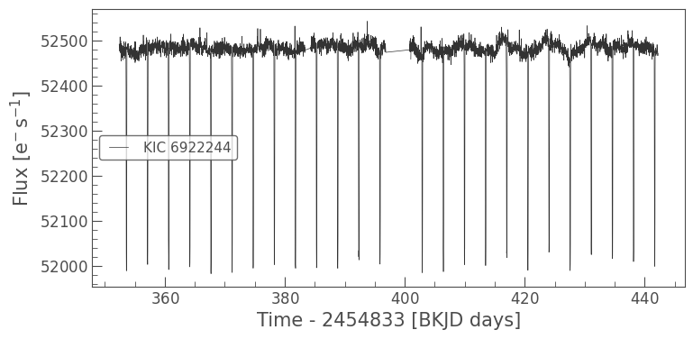
lc_Q4.plot();
Note:#
The example given above also works for downloading target pixel files (TPFs). This will produce a TargetPixelFileCollection object instead.
3. Investigating the Data#
Let’s first have a look at how these observations differ from one another. We can plot the simple aperture photometry (SAP) flux of all of the observations in the `LightCurveCollection <https://docs.lightkurve.org/reference/api/lightkurve.collections.LightCurveCollection.html#lightkurve.collections.LightCurveCollection>`__ to see how they compare.
[6]:
ax = lc_collection[0].plot(column='sap_flux', label=None)
for lc in lc_collection[1:]:
    lc.plot(ax=ax, column='sap_flux', label=None)
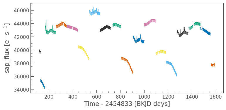
In the figure above, each quarter of data looks strikingly different, with global patterns repeating every four quarters as Kepler has made a full rotation.
The change in flux within each quarter is in part driven by changes in the telescope focus, which are caused by changes in the temperature of Kepler’s components as the spacecraft orbits the Sun. The changes are also caused by an effect called differential velocity aberration (DVA), which causes stars to drift over the course of a quarter, depending on their distance from the center of Kepler’s field of view.
While the figure above looks messy, all the systematic effects mentioned above are well understood, and have been detrended in the PDCSAP flux. For a more detailed overview, see the Kepler Data Characteristics Handbook, specifically: Section 5. Ongoing Phenomena.
4. Normalizing a Light Curve#
If we want to see the actual variation of the targeted object over the course of these observations, the plot above isn’t very useful to us. It is also not useful to have flux expressed in physical units, because it is affected by the observing conditions such as telescope focus and pointing (see above).
Instead, it is a common practice to normalize light curves by dividing by their median value. This means that the median of the newly normalized light curve will be equal to 1, and that the relative size of signals in the observation (such as transits) will be maintained.
A normalization can be performed using the normalize() method of a KeplerLightCurve, for example:
[7]:
lc_collection[4].normalize().plot();
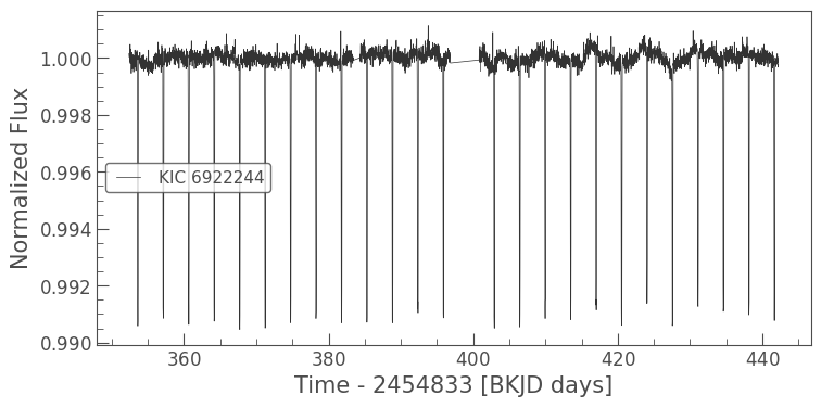
In the figure above, we have plotted the normalized PDCSAP flux for Quarter 4. The median normalized flux is at 1, and the transit depths lie around 0.991, indicating a 0.9% dip in brightness due to the planet transiting the star.
The LightCurveCollection also has a plot() method. We can use it to plot the PDCSAP flux. The method automatically normalizes the flux in same way we did for a single quarter above.
[8]:
lc_collection.plot();
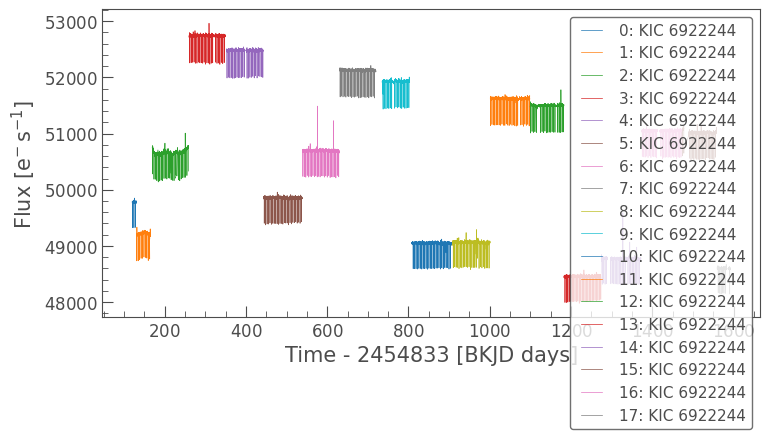
As you can see above, because we have normalized the data, all of the observations form a single consistent light curve.
5. Combining Multiple Observations into a Single Light Curve#
Finally, we can combine these different light curves into a single KeplerLightCurve object. This is done using the stitch() method. This method concatenates all quarters in our LightCurveCollection together, and normalizes them at the same time, in the manner we saw above.
[9]:
lc_stitched = lc_collection.stitch()
lc_stitched
[9]:
| time | flux | flux_err | quality | timecorr | centroid_col | centroid_row | cadenceno | sap_flux | sap_flux_err | sap_bkg | sap_bkg_err | pdcsap_flux | pdcsap_flux_err | sap_quality | psf_centr1 | psf_centr1_err | psf_centr2 | psf_centr2_err | mom_centr1 | mom_centr1_err | mom_centr2 | mom_centr2_err | pos_corr1 | pos_corr2 |
|---|---|---|---|---|---|---|---|---|---|---|---|---|---|---|---|---|---|---|---|---|---|---|---|---|
| d | pix | pix | electron / s | electron / s | electron / s | electron / s | electron / s | electron / s | pix | pix | pix | pix | pix | pix | pix | pix | pix | pix | ||||||
| Time | float32 | float32 | int32 | float32 | float64 | float64 | int32 | float32 | float32 | float32 | float32 | float32 | float32 | int32 | float64 | float32 | float64 | float32 | float64 | float32 | float64 | float32 | float32 | float32 |
| 120.53979406206781 | 1.0002389e+00 | 1.7835133e-04 | 0 | 1.641642e-03 | 676.76061 | 192.21102 | 568 | 4.0029211e+04 | 7.1942086e+00 | 1.3501000e+03 | 6.9019127e-01 | 4.9790078e+04 | 8.8780060e+00 | 0 | ——— | ——— | ——— | ——— | 676.76061 | 2.4257520e-04 | 192.21102 | 2.8915040e-04 | -6.1361594e-03 | 1.2139007e-02 |
| 120.56022845695406 | 1.0000123e+00 | 1.7952095e-04 | 0 | 1.642437e-03 | 676.76010 | 192.21002 | 569 | 4.0014566e+04 | 7.1924801e+00 | 1.3488469e+03 | 6.8939346e-01 | 4.9778801e+04 | 8.9362278e+00 | 0 | ——— | ——— | ——— | ——— | 676.76010 | 2.4263318e-04 | 192.21002 | 2.8926603e-04 | -6.3053877e-03 | 1.1505429e-02 |
| 120.58066275172314 | 9.9970073e-01 | 1.7981241e-04 | 0 | 1.643232e-03 | 676.76146 | 192.20988 | 570 | 4.0000406e+04 | 7.1918778e+00 | 1.3513733e+03 | 6.8988037e-01 | 4.9763289e+04 | 8.9507360e+00 | 0 | ——— | ——— | ——— | ——— | 676.76146 | 2.4270279e-04 | 192.20988 | 2.8932444e-04 | -5.5118860e-03 | 1.1369802e-02 |
| 120.60109724637005 | 1.0002698e+00 | 1.7900635e-04 | 0 | 1.644026e-03 | 676.76139 | 192.20938 | 571 | 4.0018668e+04 | 7.1936789e+00 | 1.3461132e+03 | 6.8999070e-01 | 4.9791617e+04 | 8.9106121e+00 | 0 | ——— | ——— | ——— | ——— | 676.76139 | 2.4260787e-04 | 192.20938 | 2.8922342e-04 | -5.5788676e-03 | 1.0246177e-02 |
| 120.62153164102347 | 1.0001223e+00 | 1.7974019e-04 | 0 | 1.644821e-03 | 676.76213 | 192.20898 | 572 | 4.0008617e+04 | 7.1923513e+00 | 1.3499850e+03 | 6.9054097e-01 | 4.9784277e+04 | 8.9471407e+00 | 0 | ——— | ——— | ——— | ——— | 676.76213 | 2.4259168e-04 | 192.20898 | 2.8918759e-04 | -4.6821944e-03 | 1.0072310e-02 |
| 120.6419659354433 | 9.9984479e-01 | 1.7990815e-04 | 0 | 1.645615e-03 | 676.76170 | 192.20871 | 573 | 3.9994742e+04 | 7.1914024e+00 | 1.3490905e+03 | 6.8729931e-01 | 4.9770461e+04 | 8.9555016e+00 | 0 | ——— | ——— | ——— | ——— | 676.76170 | 2.4268354e-04 | 192.20871 | 2.8930244e-04 | -4.2848983e-03 | 9.4073853e-03 |
| ... | ... | ... | ... | ... | ... | ... | ... | ... | ... | ... | ... | ... | ... | ... | ... | ... | ... | ... | ... | ... | ... | ... | ... | ... |
| 1590.900002857561 | 9.9988633e-01 | 1.8179342e-04 | 0 | 1.018638e-03 | 676.80148 | 192.10108 | 72526 | 3.7831559e+04 | 6.9085450e+00 | 1.2787664e+03 | 5.9414190e-01 | 4.8594551e+04 | 8.8351736e+00 | 0 | 676.75930 | 1.4916631e-04 | 192.31896 | 1.9152595e-04 | 676.80148 | 2.5232948e-04 | 192.10108 | 2.5263420e-04 | -4.0509203e-03 | 1.4821382e-02 |
| 1590.9204372017994 | 9.9999821e-01 | 1.8173133e-04 | 0 | 1.019482e-03 | 676.80166 | 192.10131 | 72527 | 3.7836602e+04 | 6.9087906e+00 | 1.2786053e+03 | 5.9385866e-01 | 4.8599988e+04 | 8.8321562e+00 | 0 | 676.75946 | 1.4911903e-04 | 192.31899 | 1.9154462e-04 | 676.80166 | 2.5230341e-04 | 192.10131 | 2.5262410e-04 | -4.0993756e-03 | 1.4611045e-02 |
| 1590.9408717461629 | 9.9969560e-01 | 1.8179418e-04 | 0 | 1.020326e-03 | 676.80144 | 192.10146 | 72528 | 3.7825430e+04 | 6.9083652e+00 | 1.2797456e+03 | 5.9316140e-01 | 4.8585281e+04 | 8.8352108e+00 | 0 | 676.75953 | 1.4916577e-04 | 192.31908 | 1.9160371e-04 | 676.80144 | 2.5239564e-04 | 192.10146 | 2.5271456e-04 | -3.9369571e-03 | 1.4928485e-02 |
| 1590.9613061904092 | 9.9994302e-01 | 1.8176372e-04 | 0 | 1.021170e-03 | 676.80124 | 192.10091 | 72529 | 3.7834938e+04 | 6.9087672e+00 | 1.2764705e+03 | 5.9434044e-01 | 4.8597305e+04 | 8.8337307e+00 | 0 | 676.75914 | 1.4914536e-04 | 192.31884 | 1.9145805e-04 | 676.80124 | 2.5227590e-04 | 192.10091 | 2.5260207e-04 | -4.1014180e-03 | 1.4680510e-02 |
| 1590.9817405346475 | 1.0001228e+00 | 1.8151020e-04 | 0 | 1.022015e-03 | 676.80224 | 192.10165 | 72530 | 3.7828816e+04 | 6.9086733e+00 | 1.2774485e+03 | 5.9289569e-01 | 4.8606039e+04 | 8.8214092e+00 | 0 | 676.75981 | 1.4909096e-04 | 192.31980 | 1.9197758e-04 | 676.80224 | 2.5231845e-04 | 192.10165 | 2.5264811e-04 | -3.6829417e-03 | 1.6025381e-02 |
| 1591.0021750787782 | 9.9999636e-01 | 1.8174112e-04 | 0 | 1.022859e-03 | 676.80192 | 192.10123 | 72531 | 3.7825363e+04 | 6.9084020e+00 | 1.2774999e+03 | 5.9428430e-01 | 4.8599898e+04 | 8.8326321e+00 | 0 | 676.75964 | 1.4915710e-04 | 192.31887 | 1.9161010e-04 | 676.80192 | 2.5232456e-04 | 192.10123 | 2.5267553e-04 | -3.9303382e-03 | 1.5094034e-02 |
This returns a single KeplerLightCurve! It is in all ways identical to KeplerLightCurve of a single quarter, just longer. We can plot it the usual way.
[10]:
lc_stitched.plot();
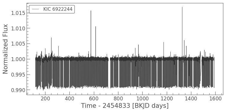
In this final normalized light curve, the interesting observational features of the star are more clear. Specifically: repeating transits that can be used to characterize planets and a noisy stellar flux that can be used to study brightness variability through asteroseismology.
Normalizing individual Kepler Quarters before combining them to form a single light curve isn’t the only way to make sure different quarters are consistent with one another. For a breakdown of other available methods and their benefits, see Section 6. Stitching Kepler Quarters Together in Kinemuchi et al. 2012.
About this Notebook#
Authors: Oliver Hall (oliver.hall@esa.int), Geert Barentsen
Updated On: 2020-09-15
Citing Lightkurve and Astropy#
If you use lightkurve or astropy for published research, please cite the authors. Click the buttons below to copy BibTeX entries to your clipboard.
[11]:
lk.show_citation_instructions()
[11]:
When using Lightkurve, we kindly request that you cite the following packages:
- lightkurve
- astropy
- astroquery — if you are using search_lightcurve() or search_targetpixelfile().
- tesscut — if you are using search_tesscut().


