What are LightCurve objects?#
LightCurve objects are data objects which encapsulate the brightness of a star over time. They provide a series of common operations, for example folding, binning, plotting, etc. There are a range of subclasses of LightCurve objects specific to telescopes, including KeplerLightCurve for Kepler and K2 data and TessLightCurve for TESS data.
Although lightkurve was designed with Kepler, K2 and TESS in mind, these objects can be used for a range of astronomy data.
You can create a LightCurve object from a TargetPixelFile object using Simple Aperture Photometry (see our tutorial for more information on Target Pixel Files here. Aperture Photometry is the simple act of summing up the values of all the pixels in a pre-defined aperture, as a function of time. By carefully choosing the shape of the aperture mask, you can avoid nearby contaminants or improve the strength of
the specific signal you are trying to measure relative to the background.
To demonstrate, lets create a KeplerLightCurve from a KeplerTargetPixelFile.
[1]:
from lightkurve import search_targetpixelfile
# First we open a Target Pixel File from MAST, this one is already cached from our previous tutorial!
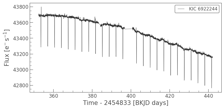
tpf = search_targetpixelfile('KIC 6922244', author="Kepler", cadence="long", quarter=4).download()
# Then we convert the target pixel file into a light curve using the pipeline-defined aperture mask.
lc = tpf.to_lightcurve(aperture_mask=tpf.pipeline_mask)
We’ve built a new KeplerLightCurve object called lc. Note in this case we’ve passed an aperture_mask to the to_lightcurve method. The default is to use the Kepler pipeline aperture. (You can pass your own aperture, which is a boolean numpy array.) By summing all the pixels in the aperture we have created a
Simple Aperture Photometry (SAP) lightcurve.
KeplerLightCurve has many useful functions that you can use. As with Target Pixel Files you can access the meta data very simply:
[2]:
lc.meta['MISSION']
[2]:
'Kepler'
[3]:
lc.meta['QUARTER']
[3]:
4
And you still have access to time and flux attributes. In a light curve, there is only one flux point for every time stamp:
[4]:
lc.time
[4]:
<Time object: scale='tdb' format='bkjd' value=[352.37632485 352.39675805 352.43762445 ... 442.16263546 442.18306983
 442.2035041 ]>
[5]:
lc.flux
[5]:
You can also check the Combined Differential Photometric Precision (“CDPP”) noise metric of the lightcurve using the built in method estimate_cdpp():
[6]:
lc.estimate_cdpp()
[6]:
Now we can use the built in plot function on the KeplerLightCurve object to plot the time series. You can pass plot any keywords you would normally pass to matplotlib.pyplot.plot.
[7]:
%matplotlib inline
lc.plot();
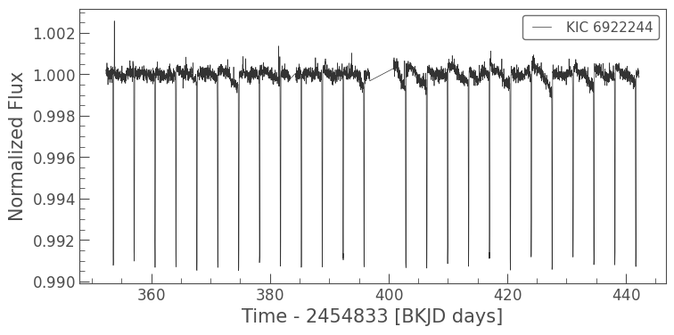
There are a set of useful functions in LightCurve objects which you can use to work with the data. These include:
flatten(): Remove long term trends using a Savitzky–Golay filter
remove_outliers(): Remove outliers using simple sigma clipping
remove_nans(): Remove infinite or NaN values (these can occur during thruster firings)
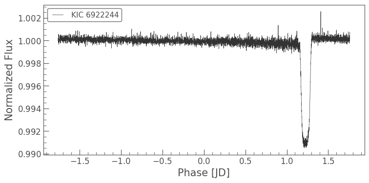
fold(): Fold the data at a particular period
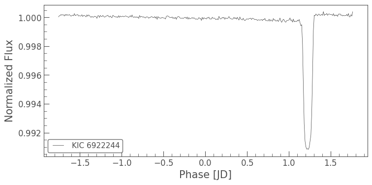
bin(): Reduce the time resolution of the array, taking the average value in each bin.
We can use these simply on a light curve object
[8]:
flat_lc = lc.flatten(window_length=401)
flat_lc.plot();
[9]:
folded_lc = flat_lc.fold(period=3.5225)
folded_lc.plot();
[10]:
binned_lc = folded_lc.bin(time_bin_size=0.01)
binned_lc.plot();
Or we can do these all in a single (long) line!
[11]:
lc.remove_nans().flatten(window_length=401).fold(period=3.5225).bin(time_bin_size=0.01).plot();
